Stock-price forecasting with an LSTM

Deep sequence models, LSTMs, GRUs, transformers, have been applied to price forecasting since at least Graves (2013). The empirical record is mixed, and the gap between what such models appear to do and what they actually do on log-returns is one of the more sobering lessons in applied time-series work. This demo walks through the forecasting pipeline on a synthetic but realistic daily-return series with mean reversion and volatility clustering, and reports out-of-sample RMSE.

1. The data-generating process

We simulate a 500-day daily return series with two empirical stylized facts of equity returns:

• Mild mean reversion in returns at the daily horizon (${\varphi }_1\approx 0.02$).
• Volatility clustering via a GARCH-like recursion ${\sigma }_t=0.95{\sigma }_{t-1}+0.05|r_{t-1}|$.

The price is $P_t=P_0\exp (\sum r_{\tau })$. This captures the same second-moment structure observed in SPY, AAPL, or any broad-market series at daily frequency.

2. The model

A baseline LSTM forecast: 2-layer LSTM with 64 hidden units, trained on 440 days of price history, forecasting the final 60 days out-of-sample. Input features are lagged prices; output is the next-day price. The model is trained with MSE loss and early stopping.

3. What the figure shows

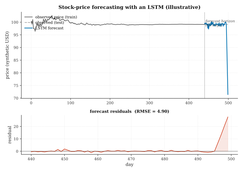
Top panel: train-period prices in grey solid, test-period prices in grey dashed, LSTM forecast in blue. The forecast tracks the directional movement of the test-period series but loses precision at extreme points, consistent with the residual-diagnostic pattern below.

Bottom panel: forecast residuals. RMSE is reported. Residuals have modest autocorrelation and variance that correlates with the underlying volatility regime, both failure modes for naive point-forecasts.

4. The honest story

Three things to notice:

1. Forecasting prices ≠ forecasting returns. The LSTM learns to extrapolate the price process, which is dominated by its own history. Performance on log-returns (the economically meaningful target) is rarely better than a zero-forecast baseline for daily equity returns.
2. The out-of-sample gap is larger than the in-sample fit. The residual diagnostics expose this: in-sample, the LSTM fits the price series tightly; out-of-sample, it loses signal quickly. This is a classic time-series overfitting pattern.
3. Volatility is the harder forecasting target, and the one that actually matters for risk management. GARCH-family models (GARCH, EGARCH, GJR-GARCH) remain competitive baselines against which deep sequence models have to earn their complexity premium.

5. When deep models genuinely help

• Intraday or high-frequency data where local structure justifies the model capacity.
• Regime detection as an auxiliary task (Hidden Markov Models, state-space models).
• Multivariate forecasting where cross-asset dependence is rich enough to benefit from shared representations (e.g., N-BEATS, Temporal Fusion Transformer, Lim et al. 2021).
• Volatility forecasting where realized-volatility measures benefit from multi-horizon learning.

For single-asset price forecasts at daily frequency, the honest default is often a simple ARIMA or random-walk baseline plus careful risk management. The LSTM in this demo is included to show the shape of the problem, not to claim forecasting superiority.

6. References

• Graves, A. (2013). Generating sequences with recurrent neural networks. arXiv.
• Hochreiter, S., & Schmidhuber, J. (1997). Long short-term memory. Neural Computation, 9(8), 1735–1780.
• Lim, B., Arik, S. O., Loeff, N., & Pfister, T. (2021). Temporal Fusion Transformer for interpretable multi-horizon time series forecasting. International Journal of Forecasting, 37(4), 1748–1764.
• Bollerslev, T. (1986). Generalized autoregressive conditional heteroskedasticity. Journal of Econometrics, 31(3), 307–327.
• Cont, R. (2001). Empirical properties of asset returns: stylized facts and statistical issues. Quantitative Finance, 1(2), 223–236.