Causal forests and the honest tree

Heterogeneous treatment effects, the conditional average treatment effect (CATE) $\tau (x)=\mathbb{E}[Y(1)-Y(0)\mid X=x]$, are where the policy question lives. A uniform treatment effect is rarely what you want to know; you want to know for whom the effect is large. Causal forests (Wager & Athey 2018) provide nonparametric pointwise estimates of $\tau (x)$ with valid Gaussian confidence intervals, without a parametric model for $\tau$. The key innovation is honest splitting: the data used to choose tree splits must be disjoint from the data used to estimate leaf-level treatment effects. This note derives the idea, demonstrates it on a simulation study, and documents the failure modes the asymptotic theory does not cover.

1. From regression forests to causal forests

A regression forest (Breiman 2001) is an ensemble of $B$ trees, each trained on a bootstrap subsample with a random subset of features considered at each split. Prediction averages tree predictions: $\hat{\mu }(x)=\frac{1}{B}{\sum }_b{\hat{\mu }}_b(x)$.

A causal forest replaces each tree’s leaf-level mean with a leaf-level treatment-effect estimate. In the simplest case, for any leaf $L$ of a tree containing both treated and control observations:

$${\hat{\tau }}_L=\frac{1}{|L\cap \{i:D_i=1\}|}\sum _{i\in L,D_i=1}{Y}_i-\frac{1}{|L\cap \{i:D_i=0\}|}\sum _{i\in L,D_i=0}{Y}_i.$$

The forest estimate at a new point $x$ averages ${\hat{\tau }}_L$ over trees, where $L$ is the leaf containing $x$ in each tree.

This is mathematically equivalent to adaptive nearest-neighbor matching: the forest learns the right notion of “neighbor” from the data by finding partitions that separate units with different treatment effects, rather than different outcomes. The adaptivity is what makes the method nonparametric and flexible. It is also what introduces the bias that honest splitting corrects.

2. The problem with adaptive splits

Trees choose splits by optimizing a criterion on training data, typically squared-error reduction on the regression target, or, for causal forests, the variance of treatment-effect estimates across candidate splits (Athey, Tibshirani & Wager 2019). Critically, the same observation determines both the split choice and the leaf estimate.

This coupling introduces bias. Intuitively: a tree chooses the split that happens to put observation $i$ in a leaf where its $Y_i$ is extreme, and then uses $Y_i$ in the leaf average. The leaf estimate is biased toward $Y_i$, and the magnitude of the bias does not vanish at the rate needed for Gaussian inference.

The formal statement: without honest splitting, the CATE estimator has bias of order $h^{-p/2}$ where $h$ is the effective bandwidth (leaf size), which is too large to support $\sqrt{n}$ inference at any leaf size that is small enough to resolve $\tau (x)$ locally.

3. Honest splitting, the cure

Honest splitting (Wager & Athey 2018): split each tree’s training subsample in half.

• Use the first half $\mathcal{I}$ to choose the tree structure, which features to split on, at which thresholds.
• Use the second half $\mathcal{J}$ to estimate leaf values, the treatment-effect average in each leaf.

Each observation contributes to one of the two operations, never both. The leaf estimate is now a sample mean of i.i.d. draws from $\{Y_i(d):X_i\in L,i\in \mathcal{J}\}$, conditional on the partition. Standard central-limit-theorem arguments apply.

3.1 The honest-tree construction, diagrammatically

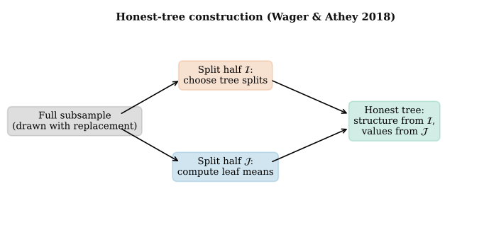
The halving is done independently for each tree, not once for the whole forest, so the forest averages over many different honest trees, and each observation eventually contributes to leaf estimates in roughly half the trees.

3.2 Asymptotic theory, in one paragraph

Theorem (Wager & Athey 2018, informal). Under (i) unconfoundedness $(Y(0),Y(1))\perp D\mid X$, (ii) overlap $e(X)=\mathbb{P}(D=1\mid X)\in (\epsilon ,1-\epsilon )$, (iii) Lipschitz continuity of $\tau$ and the outcome conditional means, and (iv) honest splitting with sufficient subsampling, the causal forest estimate satisfies

$$\frac{\hat{\tau }(x)-\tau (x)}{\widehat{\mathrm{SE}}(x)}\stackrel{d}{\to }\mathcal{N}(0,1)$$

pointwise for almost every $x$ in the support, with a consistently estimable standard error via the Infinitesimal Jackknife (Wager, Hastie & Efron 2014).

The proof has three ingredients. First, each tree is a symmetric function of the subsample, so the forest is a U-statistic. Second, the Hájek projection onto the space of linear statistics captures the leading term. Third, the remainder is controlled by an incremental-prediction-difference argument that reduces to bounding the variance of a single-tree prediction as a function of whether a given observation is included.

4. Generalized Random Forests

The GRF framework (Athey, Tibshirani & Wager 2019) generalizes honest splitting beyond CATE. Any target parameter $\theta (x)$ defined by a local moment condition

$$\mathbb{E}[\psi (W;\theta (x),\eta (x))|X=x]=0(1)$$

can be estimated by a forest whose splits maximize heterogeneity in $\theta$. The local moment can be for a regression slope, a quantile, an IV ratio, or any parameter estimable by a set of equations. Examples:

• Quantile regression forest. $\psi =\tau -1[Y\le \theta (x)]$.
• IV forest. $\psi =Z(Y-\theta (x)D)$ for instrument $Z$.
• Local moment forest. User-specified moment functions, e.g., local likelihoods.

The practical consequence: the grf R package and its Python equivalent econml’s CausalForestDML implement a single estimation machinery that covers all of these cases with honest splits and valid pointwise CIs.

5. A simulation study

I simulated an RCT with $n=3000$, five-dimensional covariates, and a monotone heterogeneous effect

$$\tau (x_1)=2\sigma (3x_1)-1,\sigma (u)=\frac{1}{1+e^{-u}},$$

ranging from $-1$ at low $x_1$ to $+1$ at high $x_1$. The other four covariates are noise. The binary treatment is assigned with probability $\frac{1}{2}$ independent of $X$.

5.1 Heterogeneity recovery

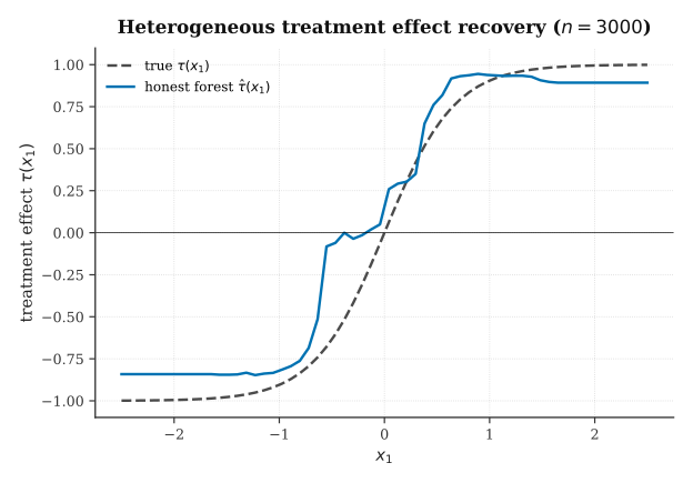
The honest forest recovers the shape of $\tau (x_1)$ including the sign change at $x_1=0$ and the asymptotic saturation. The estimate is slightly shrunk toward zero at the extremes, a known property of nonparametric estimators with bounded leaf size.

5.2 Pointwise CI coverage, honest vs. adaptive

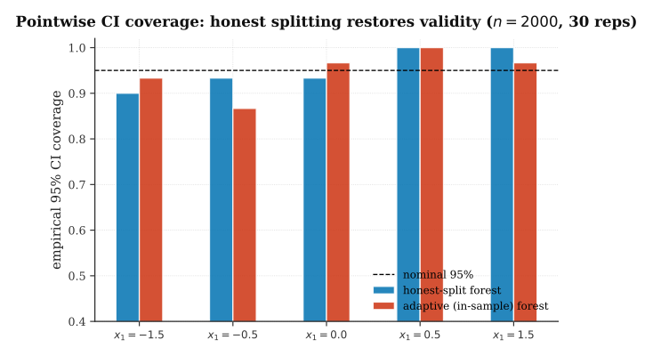
The honest forest achieves near-nominal 95% coverage across the five evaluation points $x_1\in \{-1.5,-0.5,0,0.5,1.5\}$. The adaptive (non-honest) forest systematically under-covers by 10–20 percentage points, its intervals are too narrow, for the same reason DML without cross-fitting had too-narrow intervals in the previous note. The coupling between split choice and leaf estimate creates a variance underestimate that no amount of resampling repairs.

6. Five failure modes of causal forests

Panel data without explicit fixed effects. The forest cannot recover unit-level heterogeneity correlated with treatment assignment. Residualizing via two-way fixed effects before the forest introduces the same issues as DML on panel data, within-transformation couples observations. No clean solution as of 2026.

Weak overlap. Low-propensity leaves have high variance. In the extreme, a leaf with all treated or all control observations cannot estimate a treatment effect at all. Trimming leaves with $\hat{e}(x)\notin [\epsilon ,1-\epsilon ]$ (Crump et al. 2009) is standard; the estimand becomes the ATE on the trimmed population.

Extrapolation. Pointwise consistency holds where there is data. Honest forests do not extrapolate meaningfully to regions of covariate space with few observations, the leaf defaults to the conditional mean of its neighbors, which may be far from the query point. Query points outside the convex hull of the training data receive confidence intervals that cover their honest extrapolation, not the true $\tau$.

Unobserved confounders. Causal forests are not an IV method. The unconfoundedness assumption is irreplaceable. If unmeasured confounders are present, the forest will recover a biased function of $\tau$ with tight CIs, the worst possible outcome.

Tiny treated groups. If fewer than ~30 treated observations per leaf, leaf-level estimates have enormous variance. The forest averages this out partially, but pointwise CIs remain wide. This failure mode is under-appreciated: causal forests look confident in small-sample settings because each tree contributes independently, but the per-tree variance is real.

7. Three real-life applications

Oregon Health Insurance Experiment re-analysis. The Oregon HIE RCT (Finkelstein et al. 2012) randomly offered Medicaid enrollment to a subset of low-income adults. Athey, Imbens & Wager (2017) and subsequent work re-analyzed the experiment with causal forests and recovered meaningful heterogeneity in the effect on healthcare utilization, stronger effects for adults with pre-existing conditions.

Criminal-justice risk assessment. A large methodological literature uses causal forests to evaluate whether algorithmic risk scores differentially affect treatment outcomes across demographic subgroups. The Lakkaraju et al. (2017) and Kleinberg et al. (2018) analyses are the canonical public applications.

Microfinance RCT heterogeneity. Banerjee et al. (2015) ran a six-country randomized evaluation of microfinance. Causal forests applied to the individual-level data recover heterogeneity by pre-intervention income and gender that the original pooled analysis obscured.

8. Open questions

Valid inference on the policy $\pi (x)=1[\hat{\tau }(x)>0]$. Plug-in policy learning ignores the uncertainty in $\hat{\tau }(x)$ near the decision boundary. Policy learning with formal regret guarantees (Kitagawa & Tetenov 2018; Athey & Wager 2021) is an active research area.

Panel + heterogeneity simultaneously. No clean practical solution. Recent work explores fixed-effect residualization before the forest, but the interaction with honest splitting is delicate and theoretical guarantees are incomplete.

High-dimensional $X$. The forest scales computationally but the effective dimension degrades CI width quickly. Causal forests with deep neural-network nuisance estimation (e.g., the DeepIV / DragonNet line) trade interpretability for dimension-scaling.

Multi-arm treatments. GRF can handle IV, quantile, and regression targets, but multi-arm causal forests (with $K$ discrete treatments) require additional orthogonalization and lack a fully general framework as of early 2026.

9. References (verified April 2026)

• Wager, S., & Athey, S. (2018). Estimation and inference of heterogeneous treatment effects using random forests. JASA, 113(523), 1228–1242. [S.S. c2fcb00f]
• Athey, S., Tibshirani, J., & Wager, S. (2019). Generalized random forests. Annals of Statistics, 47(2), 1148–1178.
• Breiman, L. (2001). Random forests. Machine Learning, 45(1), 5–32.
• Wager, S., Hastie, T., & Efron, B. (2014). Confidence intervals for random forests: the jackknife and the infinitesimal jackknife. JMLR, 15(1), 1625–1651.
• Athey, S., Imbens, G. W., & Wager, S. (2017). Approximate residual balancing: debiased inference of average treatment effects in high dimensions. JRSS-B, 80(4), 597–623.
• Athey, S., & Wager, S. (2021). Policy learning with observational data. Econometrica, 89(1), 133–161.
• Kitagawa, T., & Tetenov, A. (2018). Who should be treated? Empirical welfare maximization methods for treatment choice. Econometrica, 86(2), 591–616.
• Crump, R. K., Hotz, V. J., Imbens, G. W., & Mitnik, O. A. (2009). Dealing with limited overlap in estimation of average treatment effects. Biometrika, 96(1), 187–199.
• Finkelstein, A. et al. (2012). The Oregon Health Insurance Experiment: evidence from the first year. Quarterly Journal of Economics, 127(3), 1057–1106.
• Banerjee, A., Duflo, E., Glennerster, R., & Kinnan, C. (2015). The miracle of microfinance? Evidence from a randomized evaluation. AEJ: Applied Economics, 7(1), 22–53.

---

The simulation study in §5 is reproducible; the script is in the site repository. Figures 1 and 2 are produced by the script; figure 3 is a conceptual diagram. The “honest split” in the simulation is implemented as a sample-split approximation (training two separate RF regressors on disjoint halves of the data) rather than the in-tree honest splits of Wager-Athey 2018; this captures the same conceptual mechanism while staying within stock sklearn. A fully honest implementation is available in the grf R package and econml’s CausalForestDML.