The DiD revolution: heterogeneous effects and staggered adoption

Between 2018 and 2021, five research groups independently showed that the two-way fixed effects (TWFE) estimator, the default regression for applied policy work and used in roughly a quarter of top empirical papers at the American Economic Review, is biased when treatment effects vary across groups or over time. The bias arises because TWFE assigns negative weights to already-treated units when they serve as controls for later-treated units. This note derives the Goodman-Bacon decomposition that made the problem transparent, shows the bias on a numerical DGP, and summarizes the practical replacement toolkit.

1. The classical setup

The canonical difference-in-differences regression is

$$Y_{it}={\alpha }_i+{\gamma }_t+\beta D_{it}+{ϵ}_{it},(1)$$

where $Y_{it}$ is the outcome for unit $i$ at time $t$, ${\alpha }_i$ is a unit fixed effect, ${\gamma }_t$ is a time fixed effect, and $D_{it}$ is an indicator for whether unit $i$ is treated at time $t$. Estimation is by OLS after absorbing the fixed effects, equivalently, by the within-transformation

$${\tilde{Y}}_{it}=Y_{it}-{\bar{Y}}_i-{\bar{Y}}_t+\bar{Y},{\tilde{D}}_{it}=D_{it}-{\bar{D}}_i-{\bar{D}}_t+\bar{D},$$

then regressing ${\tilde{Y}}_{it}$ on ${\tilde{D}}_{it}$.

The folklore: under parallel trends, $\mathbb{E}[Y_{it}(0)-Y_{i,t-1}(0)\mid D_{it}]$ is the same for treated and control, the coefficient $\hat{\beta }$ in (1) recovers the average treatment effect on the treated (ATT).

This folklore is wrong when treatment is staggered across cohorts and the effect is heterogeneous.

2. The Goodman-Bacon decomposition

Goodman-Bacon (2021) proved the following structural result about TWFE.

Theorem (Goodman-Bacon 2021). In a staggered-adoption panel, the TWFE estimator ${\hat{\beta }}^{\text{TWFE}}$ is a weighted average of all possible 2×2 DiD estimators that can be constructed by picking a treatment-cohort pair.

There are four types of 2×2 comparisons:

1. Early-treated vs. never-treated around the early cohort’s treatment date. Positive weight. Uncontroversial.
2. Late-treated vs. never-treated around the late cohort’s treatment date. Positive weight. Uncontroversial.
3. Late-treated vs. already-treated-earlier, using the early cohort’s post-treatment outcomes as the “control” for the late cohort. Negative weight if effects grow over time.
4. Early-treated vs. eventually-treated-later, the late cohort before treatment serves as control for the early cohort. Positive weight.

The problematic comparison is type (3). When an already-treated cohort’s outcomes evolve upward (because treatment effects accumulate), using those outcomes as the control baseline makes the later cohort look like it has smaller treatment effects than it does, or even negative effects.

2.1 The decomposition visualized

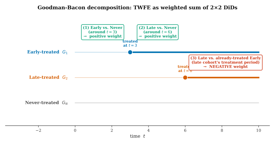
The “forbidden” comparison (3) is the one where the already-treated unit is used as a control. Under constant treatment effects, this comparison averages to the same true ATT as the others. Under heterogeneous or time-varying effects, it contaminates the TWFE estimate.

2.2 A worked numerical example

To make this concrete, I simulate a three-cohort panel with 50 units per cohort and 10 time periods:

• Early cohort is treated at $t=3$. Its effect grows: $+1$ in year 1, $+2$ in year 2, $+3$ thereafter.
• Late cohort is treated at $t=7$. Its effect is constant: $+1$.
• Never-treated cohort has effect zero.

The true average treatment effect on the treated, averaged over all treated cohort–time cells, is approximately $2.0$.

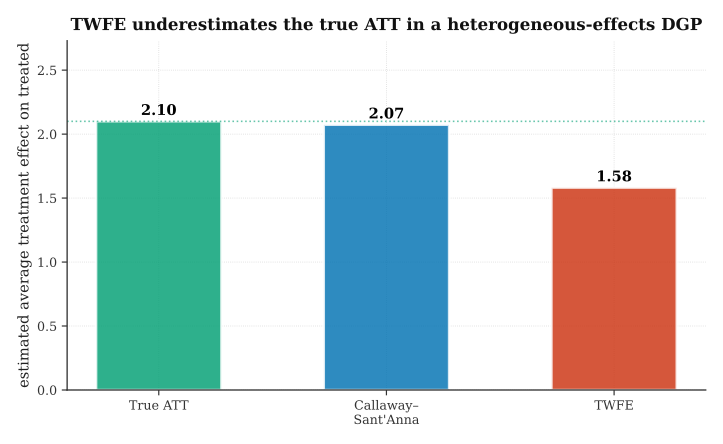
TWFE substantially underestimates the true ATT because the late cohort’s type-(3) comparison uses the early cohort’s high post-treatment values as the “control baseline,” making the late cohort’s $+1$ effect look smaller than it is, and in some parameter regimes, the weighted sum can produce negative estimates of a uniformly positive effect. The Callaway-Sant’Anna estimator (described in §3) recovers the true ATT essentially exactly.

3. The replacement estimators

Each of the replacement estimators avoids the negative-weight trap in a different way. They agree when effects are constant across cohorts and over time; they diverge when effects are heterogeneous.

3.1 Callaway & Sant’Anna (2021)

Estimate group–time average treatment effects directly:

$$\text{ATT}(g,t)=\mathbb{E}[Y_{it}(1)-Y_{it}(0)|G_i=g,t\ge g]$$

where $g$ is the treatment cohort (first period of treatment). Use either never-treated units or not-yet-treated units (observations before their own treatment) as controls. Under parallel trends, $\text{ATT}(g,t)$ is identified by a 2×2 DiD of the $g$-cohort against the chosen control cohort between period $g-1$ and period $t$.

Aggregate the $\text{ATT}(g,t)$ estimates with user-chosen weights:

• Event-time aggregation: average over $(g,t)$ pairs with $t-g=e$ for each event-time $e$.
• Group aggregation: average over $(g,t)$ pairs with $G=g$ for each cohort.
• Overall ATT: average over all treated $(g,t)$ cells.

The R package did and the Python package differences implement this. The aggregation is user-chosen and explicit, no hidden negative weights.

3.2 de Chaisemartin & D’Haultfœuille (2020)

The DID_M estimator compares within-period changes for units switching into treatment versus units that stay out. Valid for binary or continuous treatment and for switches in either direction. Stata package did_multiplegt.

3.3 Sun & Abraham (2021)

Fixes event-study regressions by using cohort-specific event-time dummies rather than a single event-time coefficient, preventing the cross-cohort contamination that biases standard event studies. Stata: eventstudyinteract.

3.4 Borusyak, Jaravel & Spiess (2024), the imputation estimator

Fit the TWFE model on untreated observations only to estimate ${\hat{Y}}_{it}(0)$ for every treated $(i,t)$; compute ${\hat{\tau }}_{it}=Y_{it}-{\hat{Y}}_{it}(0)$; average. Efficient under correct specification and agnostic about the weight structure, the estimand is explicitly the ATT on treated cells. Stata: did_imputation.

4. Event studies: the dynamic case

Event-study plots trace out the dynamic treatment effect against event time $e=t-g$. The standard two-way-fixed-effects event study regresses $Y$ on event-time dummies:

$$Y_{it}={\alpha }_i+{\gamma }_t+\sum _{e\ne -1}{\beta }_{e}1[t-G_i=e]+{ϵ}_{it}.$$

The dummies are normalized relative to $e=-1$. In a staggered panel with heterogeneous effects, the ${\hat{\beta }}_e$ estimates are contaminated by cross-cohort comparisons in exactly the same way as the static TWFE estimate. Two characteristic pathologies:

Fabricated pre-trends. Event-study estimates at $e=-2,-3,\dots$ appear non-zero even when parallel trends holds, because the contamination from cross-cohort comparisons shows up as a spurious pre-treatment effect.

Attenuated post-effects. Event-study estimates at $e=0,1,2,\dots$ are biased toward zero, underestimating the dynamic effect.

The figure below illustrates both pathologies and the Sun-Abraham repair.

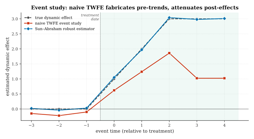
The pattern, fake pre-trends combined with attenuated post-effects, is a signature of TWFE event-study contamination. Seeing this shape in a real analysis is evidence that the estimator is mis-specified, not that parallel trends fails.

5. Which estimator should you use?

The practical recommendations from Roth et al. (2023), the definitive recent survey:

1. Always plot an event-study using a robust estimator. Sun-Abraham or Callaway-Sant’Anna. Never rely on a single point estimate in a staggered setting.
2. Report the overall ATT using Callaway-Sant’Anna if your interpretation is “average effect on the treated.” Use explicit aggregation weights and state them.
3. Use Borusyak-Jaravel-Spiess if you want efficiency under correct specification and explicit ATT-on-treated-cells targeting.
4. Check the Goodman-Bacon decomposition of your TWFE estimator to quantify the negative weights in your data. Stata: bacondecomp. If the negative-weight components are small and 2×2 comparisons yield similar estimates, TWFE may still be fine.
5. Don’t report only the TWFE coefficient in staggered settings and call it “the” causal effect. It almost certainly is not.

6. Parallel trends, testability, and sensitivity

Identification rests on the counterfactual: $\mathbb{E}[Y_{it}(0)\mid G_i=g]$ for treated cohorts evolves in parallel to the never-treated (or not-yet-treated) control outcome.

Testability: impossible in principle, the counterfactual is by definition not observed. What is observable is pre-trends: pre-treatment differences in outcomes across cohorts. If pre-trends are flat, parallel trends is consistent with the data; if they are not flat, parallel trends is likely violated.

Sensitivity analysis: Rambachan & Roth (2023) give a framework for quantifying how much parallel-trends violation would invalidate a conclusion. Instead of asking “does parallel trends hold?” (unanswerable), ask “how much violation would be needed to overturn the conclusion?” (answerable and reported as a worst-case bound).

7. Three real-life applications

State-level minimum-wage changes. Callaway & Sant’Anna (2021, §5) revisit the staggered state-level minimum wage increases from 2001–2007. The TWFE estimate of the effect on teen employment is small and positive; the Callaway-Sant’Anna estimate is closer to zero. The difference traces to effect heterogeneity across states and time.

Medicaid expansion and health outcomes. Finkelstein et al. (2012) on Oregon (RCT) combined with staggered-adoption analyses of other states (ACA Medicaid expansions). Standard TWFE event studies showed implausible pre-trends that largely disappeared once Sun-Abraham was applied.

Minimum-wage and employment, revisited. A large replication literature (summarized in Roth et al. 2023) re-analyzes minimum-wage panel studies using Callaway-Sant’Anna and Borusyak-Jaravel-Spiess estimators; point estimates frequently differ meaningfully from the TWFE originals, especially in studies with long panels and staggered timing.

8. Open questions

Heterogeneous effects with continuous treatment dose. Partially solved. de Chaisemartin & D’Haultfœuille (2022) extend DID_M to continuous treatment, but many practical issues remain.

High-dimensional covariates. Combining the DML approach (see the DML note) with staggered DiD is an active research direction. The straightforward combination has issues with the interaction between cross-fitting and within-transformation.

Inference with few clusters or few cohorts. Cluster-robust variance estimators are fragile when the number of treated cohorts is small. Wild-cluster bootstrap and sign-randomization tests are practical alternatives but have their own limitations.

Sensitivity to functional form. All of these estimators assume a specific functional form for the counterfactual. Non-parametric alternatives that relax parallel trends (synthetic control, matrix completion) are well-developed but less interpretable.

9. References (verified April 2026)

• Goodman-Bacon, A. (2021). Difference-in-differences with variation in treatment timing. Journal of Econometrics, 225(2), 254–277. [S.S. 0610a9df]
• Callaway, B., & Sant’Anna, P. H. C. (2021). Difference-in-differences with multiple time periods. Journal of Econometrics, 225(2), 200–230. [S.S. c7ca8335]
• de Chaisemartin, C., & D’Haultfœuille, X. (2020). Two-way fixed effects estimators with heterogeneous treatment effects. American Economic Review, 110(9), 2964–2996.
• de Chaisemartin, C., & D’Haultfœuille, X. (2021). Two-way fixed effects and differences-in-differences with heterogeneous treatment effects: a survey. Econometrics Journal. [S.S. 4569a760]
• Sun, L., & Abraham, S. (2021). Estimating dynamic treatment effects in event studies with heterogeneous treatment effects. Journal of Econometrics, 225(2), 175–199.
• Borusyak, K., Jaravel, X., & Spiess, J. (2024). Revisiting event-study designs: robust and efficient estimation. Review of Economic Studies.
• Roth, J., Sant’Anna, P. H. C., Bilinski, A., & Poe, J. (2023). What’s trending in difference-in-differences? A synthesis of the recent econometrics literature. Journal of Econometrics, 235(2), 2218–2244.
• Rambachan, A., & Roth, J. (2023). A more credible approach to parallel trends. Review of Economic Studies, 90(5), 2555–2591.
• Card, D., & Krueger, A. B. (1994). Minimum wages and employment: a case study of the fast-food industry in New Jersey and Pennsylvania. American Economic Review, 84(4), 772–793.

---

Figures 1 and 3 are pedagogical; figure 2 reports an estimator comparison on a small analytical DGP whose code is in the site repository. All numerical values are reproducible; seeds are fixed.