Quantile treatment effects: estimands, identification, and a panel-data pitfall

A quantile treatment effect at level $\tau$ is not the treatment effect for units at the $\tau$-th percentile of $Y$. It is the difference between the $\tau$-th quantile of the treated potential-outcome distribution and the $\tau$-th quantile of the untreated potential-outcome distribution. Firpo, Fortin & Lemieux (2009) formalized this distinction and introduced the Recentered Influence Function (RIF) regression that lets you estimate unconditional QTEs as a coefficient in an OLS regression. In panel settings, especially combined with two-way fixed effects, the conditional/unconditional distinction is often missed, with consequences for policy that are both predictable and avoidable.

1. Two QTEs, not one

The unconditional QTE at level $\tau$ is

$${\mathrm{QTE}}_{\tau }=Q_{Y(1)}(\tau )-Q_{Y(0)}(\tau ).(1)$$

It compares quantiles of the marginal distributions of the two potential outcomes. If $Y$ is wages, ${\mathrm{QTE}}_{0.5}$ is the difference in median wages between the treated and untreated worlds.

The conditional QTE at level $\tau$ and covariate $x$ is

$${\mathrm{QTE}}_{\tau }(x)=Q_{Y(1)\mid X=x}(\tau )-Q_{Y(0)\mid X=x}(\tau ).(2)$$

It compares quantiles of the potential-outcome distributions conditional on covariates.

The two are not related by simple averaging. The quantile of a marginal distribution is not the average of conditional quantiles. Formally, even if ${\mathrm{QTE}}_{\tau }(x)=\Delta$ for every $x$, the unconditional ${\mathrm{QTE}}_{\tau }$ need not equal $\Delta$, it equals $\Delta$ only when the treatment does not change the shape of the outcome distribution at all.

1.1 The distinction visualized

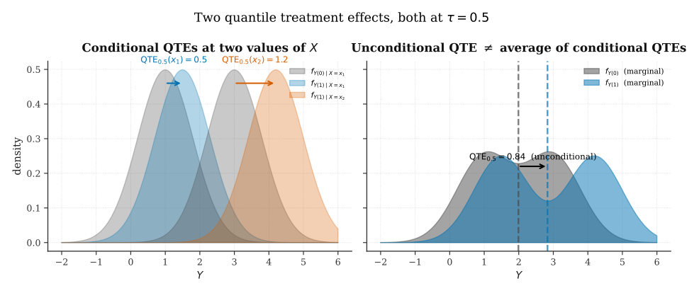
The left panel shows two values of $X$ with different conditional QTEs ($+0.5$ and $+1.2$). The right panel shows that averaging over $X$ to get the marginal distributions, the unconditional median shift is neither $0.5$ nor $1.2$ nor their average, it depends on the full mixture structure.

Consequences for practice:

• Quantile regression à la Koenker & Bassett (1978) estimates conditional quantiles. Using the coefficient as a quantile treatment effect conflates (1) and (2).
• RIF regression (§3) is the remedy: it targets (1) directly via a clever re-parameterization.

2. Conditional quantile regression, briefly

The Koenker-Bassett (1978) estimator minimizes the asymmetric check function

$${\rho }_{\tau }(u)=u(\tau -1[u<0]).$$

For a linear model $Q_{Y\mid X}(\tau )=X^{\top }\beta (\tau )$, the estimator is

$$\hat{\beta }(\tau )=\arg \underset{\beta }{\min }\sum _i{\rho }_{\tau }(Y_i-X_i^{\top }\beta ).$$

$\hat{\beta }(\tau )$ is consistent for the conditional quantile function and $\sqrt{n}$-asymptotically normal under standard regularity conditions. The coefficient on a treatment indicator $D$ in this regression estimates ${\mathrm{QTE}}_{\tau }(x)$, not ${\mathrm{QTE}}_{\tau }$. If you want (1), you need something else.

3. Firpo-Fortin-Lemieux: the RIF regression

The elegant insight: the $\tau$-th quantile is a functional of the outcome distribution $F_Y$, and its influence function has a closed form.

Definition. The influence function of the functional $\nu (F)=Q_F(\tau )=F^{-1}(\tau )$ at the distribution $F_Y$ is

$$\mathrm{IF}(y;q_{\tau },F_Y)=\frac{\tau -1[y\le q_{\tau }]}{f_Y(q_{\tau })},$$

where $q_{\tau }=Q_{F_Y}(\tau )$ and $f_Y$ is the density.

The Recentered Influence Function (RIF) is

$$\mathrm{RIF}(y;q_{\tau })=q_{\tau }+\mathrm{IF}(y;q_{\tau },F_Y)=q_{\tau }+\frac{\tau -1[y\le q_{\tau }]}{f_Y(q_{\tau })}.(3)$$

Two properties make RIF useful.

Property 1: centering. $\mathbb{E}[\mathrm{RIF}(Y;q_{\tau })]=q_{\tau }$. This follows from $\mathbb{E}[1[Y\le q_{\tau }]]=\tau$.

Property 2: linearity under mixture. For any decomposition $F_Y=\int F_{Y\mid X=x}dP(x)$ into conditional distributions,

$$q_{\tau }=\mathbb{E}[\mathrm{RIF}(Y;q_{\tau })]=\int \mathbb{E}[\mathrm{RIF}(Y;q_{\tau })\mid X=x]dP(x).$$

So the unconditional $\tau$-th quantile decomposes into an integral of the conditional expectation of the RIF, which is a regression problem. Fit a linear model $\mathbb{E}[\mathrm{RIF}(Y;q_{\tau })\mid X,D]=X^{\top }\gamma (\tau )+\delta (\tau )D$ by OLS; the coefficient $\hat{\delta }(\tau )$ is a consistent estimate of the unconditional QTE at $\tau$ (with a causal interpretation under unconfoundedness).

3.1 The RIF visualized

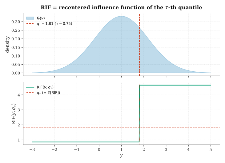
The RIF is a step function that equals $q_{\tau }-(1-\tau )/f(q_{\tau })$ below the quantile and $q_{\tau }+\tau /f(q_{\tau })$ above. Its expectation under $F_Y$ is exactly $q_{\tau }$. When you regress the RIF on covariates, you are decomposing the movement of the quantile under a perturbation in the covariate distribution.

3.2 The RIF regression procedure

1. Estimate ${\hat{q}}_{\tau }$ as the sample $\tau$-quantile.
2. Estimate ${\hat{f}}_Y({\hat{q}}_{\tau })$ by a kernel density.
3. Compute ${\widehat{\mathrm{RIF}}}_i={\hat{q}}_{\tau }+(\tau -1[Y_i\le {\hat{q}}_{\tau }])/{\hat{f}}_Y({\hat{q}}_{\tau })$ for each observation.
4. Regress ${\widehat{\mathrm{RIF}}}_i$ on $X_i$ and $D_i$ by OLS.
5. The coefficient on $D$ is the unconditional QTE at $\tau$.

The standard error from the OLS regression is not directly valid, it ignores the uncertainty in ${\hat{q}}_{\tau }$ and ${\hat{f}}_Y({\hat{q}}_{\tau })$. Robust alternatives include bootstrap-all-steps or the analytical correction in Firpo, Fortin & Lemieux (2009).

4. QTE identification under unconfoundedness

Assume $(Y(0),Y(1))\perp D\mid X$ (unconfoundedness) and overlap $0<e(X)=\mathbb{P}(D=1\mid X)<1$. Then

$$F_{Y(d)}(y)=\int F_{Y\mid D=d,X=x}(y)dP(x)\text{for }d\in \{0,1\},$$

i.e., the potential-outcome CDF is identified by averaging conditional CDFs. Invert to get $Q_{Y(d)}(\tau )$. The unconditional QTE (1) is then identified.

Practical implementation: estimate the conditional CDFs by distributional regression or kernel smoothing, weight by inverse-propensity $1/\hat{e}(X)$ or $1/(1-\hat{e}(X))$, integrate, then invert. Chernozhukov, Fernández-Val & Melly (2013) give a general framework. Chernozhukov & Hansen (2005) provide an IV extension.

5. The panel-data pitfall

In panel settings with unit fixed effects, researchers often run conditional quantile regressions with unit dummies and interpret the coefficient as the effect on units at the $\tau$-th percentile. This is a common mistake with a specific structure.

Consider a simple panel $Y_{it}={\alpha }_i+{\gamma }_t+\beta D_{it}+{ϵ}_{it}$. The within-transformed outcome ${\tilde{Y}}_{it}=Y_{it}-{\bar{Y}}_i-{\bar{Y}}_t+\bar{Y}$ has a very different distribution from the raw $Y_{it}$. Running quantile regression on ${\tilde{Y}}_{it}$ and interpreting the coefficient as “the effect on the top decile of $Y$” is a category error: the top decile of $\tilde{Y}$ is not the top decile of $Y$.

5.1 The two subpopulations are different

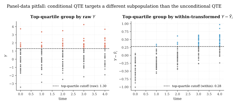
The left panel highlights the top-quartile group defined by raw $Y$; the right panel highlights the top-quartile group defined by the within-transformed $\tilde{Y}=Y-{\bar{Y}}_i$. The two groups barely overlap. A policy “target the top quartile” means something different in each case, and a quantile treatment effect estimated on within-transformed data tells you about the second group, not the first.

The pitfall is asymmetric: if effects are monotone in baseline $Y$, the naive approach can assign the largest estimated $\tau$-QTE to the wrong end of the distribution. This reasoning error has been documented in applied work to produce policy recommendations that systematically target the wrong subpopulation.

5.2 The right tool for panel QTEs

Callaway & Li (2019) extend the Callaway-Sant’Anna DiD framework to quantile treatment effects on the treated. The estimand is

$$\mathrm{QTT}(g,t;\tau )=Q_{Y_t(g)\mid G=g}(\tau )-Q_{Y_t(0)\mid G=g}(\tau ),$$

i.e., the $\tau$-th quantile of the treatment effect on cohort $g$ at period $t$. Identification uses a copula stability assumption in place of parallel trends, which is well-suited to settings where the entire distribution matters, inequality-oriented policy evaluation, for instance. The method recovers the dynamic distributional effect of treatment on the treated without conflating conditional and unconditional estimands.

6. Three real-life applications

Wage decomposition and the gender wage gap. Firpo, Fortin & Lemieux (2011) apply RIF regression to Current Population Survey data to decompose the change in the U.S. gender wage gap across the distribution. The bottom-decile gap is driven by different factors than the top-decile gap, a finding invisible to conditional quantile regression.

Inequality effects of education. Lemieux (2006) uses RIF-OLS to decompose increases in wage inequality into components from rising returns to education vs. rising residual inequality. The RIF framework is essential because the object of interest, the $90/10$ wage ratio, is a functional of the marginal distribution.

Microcredit distributional effects. Banerjee et al. (2015) and subsequent work use quantile treatment effects on microfinance RCT data to show that the average effect of microcredit is near zero but there are meaningful positive effects in the upper tail and negligible effects in the lower tail. The unconditional QTE framework is the right tool for exactly this question.

7. Open questions

Continuous-treatment quantile heterogeneity. RIF regression is designed for binary or discrete treatment. Continuous-treatment QTEs require different machinery (quantile partial effects, Chernozhukov, Fernández-Val & Kowalski 2015).

DML for quantile targets. Semenova & Chernozhukov (2021) cover CATE but the unconditional QTE target has not been integrated cleanly with the DML framework. An open methodological direction.

Finite-sample inference. RIF regression is sensitive to the density-at-quantile estimate ${\hat{f}}_Y({\hat{q}}_{\tau })$. Robust alternatives (distribution regression, M-quantile regression) are available but trade off interpretability.

Multivariate QTEs. When the outcome is multivariate (e.g., wage and hours), the notion of “the $\tau$-th quantile” becomes multivariate. Depth-based and copula-based extensions exist but lack a unified framework.

8. References (verified April 2026)

• Firpo, S., Fortin, N. M., & Lemieux, T. (2009). Unconditional quantile regressions. Econometrica, 77(3), 953–973.
• Firpo, S., Fortin, N. M., & Lemieux, T. (2011). Decomposition methods in economics. Handbook of Labor Economics, 4A, 1–102.
• Koenker, R., & Bassett, G. (1978). Regression quantiles. Econometrica, 46(1), 33–50.
• Koenker, R. (2005). Quantile regression. Cambridge University Press.
• Chernozhukov, V., & Hansen, C. (2005). An IV model of quantile treatment effects. Econometrica, 73(1), 245–261.
• Chernozhukov, V., Fernández-Val, I., & Melly, B. (2013). Inference on counterfactual distributions. Econometrica, 81(6), 2205–2268.
• Chernozhukov, V., Fernández-Val, I., & Kowalski, A. E. (2015). Quantile regression with censoring and endogeneity. Journal of Econometrics, 186(1), 201–221.
• Callaway, B., & Li, T. (2019). Quantile treatment effects in difference in differences models with panel data. Quantitative Economics, 10(4), 1579–1618.
• Lemieux, T. (2006). Increasing residual wage inequality: composition effects, noisy data, or rising demand for skill? American Economic Review, 96(3), 461–498.
• Banerjee, A., Duflo, E., Glennerster, R., & Kinnan, C. (2015). The miracle of microfinance? Evidence from a randomized evaluation. AEJ: Applied Economics, 7(1), 22–53.

---

Figures produced by reproducible Python scripts in the site repository. All illustrations are analytical / small-simulation; no benchmark datasets are used, for both pedagogical clarity and reproducibility.