Conformal prediction: distribution-free uncertainty that finally works

Given any prediction model, linear, random forest, transformer, black box, conformal prediction wraps its output in a set that is guaranteed to contain the true label with user-specified probability $1-\alpha$, under only the exchangeability assumption on the calibration data. No distribution assumption. No model-correctness assumption. The guarantee is finite-sample and marginal. This note derives split conformal prediction from first principles, explains the crucial distinction between marginal and conditional coverage, and covers two extensions (conformalized quantile regression and adaptive conformal inference under distribution shift) that made conformal practical.

1. The setup and the promise

We have data $(X_1,Y_1),\dots ,(X_n,Y_n),(X_{n+1},Y_{n+1})$ all exchangeable, i.e., their joint distribution is invariant under permutations. We observe the first $n$ pairs and the covariate $X_{n+1}$. Our goal is to output a prediction set ${\hat{C}}_{\alpha }(X_{n+1})\subseteq \mathcal{Y}$ with

$$\mathbb{P}(Y_{n+1}\in {\hat{C}}_{\alpha }(X_{n+1}))\ge 1-\alpha .(1)$$

Three properties of (1) deserve emphasis.

Finite-sample. The inequality holds for every $n$, not in some asymptotic limit. It holds at $n=20$ exactly as it holds at $n=10^6$.

Distribution-free. No assumption on the joint distribution of $(X,Y)$ beyond exchangeability of the data. The true distribution can be wildly non-Gaussian, heavy-tailed, multimodal, or depend on $X$ in any way.

Model-agnostic. The guarantee does not depend on the prediction model being correctly specified, or even particularly accurate. A terrible model gives a wide, valid set; a great model gives a tight, useful set. The method extracts the uncertainty information from the calibration data, not from the model.

The probability in (1) is marginal, averaged over both $X_{n+1}$ and the entire data-generation process. This will matter.

2. Split conformal prediction in a single algorithm

The simplest and most widely used conformal variant is split conformal (Papadopoulos et al. 2002; Vovk et al. 2005).

Split conformal, the algorithm:

1. Randomly split the data into a training fold ${\mathcal{I}}_{\mathrm{tr}}$ and a calibration fold ${\mathcal{I}}_{\mathrm{cal}}$ (typically 50/50 or 70/30).
2. Fit any predictor $\hat{\mu }$ on ${\mathcal{I}}_{\mathrm{tr}}$.
3. For each calibration point $i\in {\mathcal{I}}_{\mathrm{cal}}$, compute a nonconformity score $s_i=s(X_i,Y_i,\hat{\mu })$. For regression: $s_i=|Y_i-\hat{\mu }(X_i)|$. For classification: $s_i=1-{\hat{\mu }}_{y_i}(X_i)$ where ${\hat{\mu }}_y$ is the predicted probability of class $y$.
4. Let $\hat{q}$ be the $\lceil (n_{\mathrm{cal}}+1)(1-\alpha )\rceil /n_{\mathrm{cal}}$ empirical quantile of $\{s_i{\}}_{i\in {\mathcal{I}}_{\mathrm{cal}}}$.
5. Output ${\hat{C}}_{\alpha }(X_{n+1})=\{y\in \mathcal{Y}:s(X_{n+1},y,\hat{\mu })\le \hat{q}\}$.

Guarantee (Vovk, Gammerman & Shafer 2005): Under exchangeability of the calibration data and the test point,

$$\mathbb{P}(Y_{n+1}\in {\hat{C}}_{\alpha }(X_{n+1}))\ge 1-\alpha ,$$

with equality in the continuous-score case.

2.1 The two-line proof

Exchangeability implies that the nonconformity score $s_{n+1}:=s(X_{n+1},Y_{n+1},\hat{\mu })$ is exchangeable with $s_1,\dots ,s_{n_{\mathrm{cal}}}$. Therefore,

$$\mathbb{P}(s_{n+1}\le s_{(k)})=\frac{k}{n_{\mathrm{cal}}+1}$$

where $s_{(k)}$ is the $k$-th order statistic. Choose $k=\lceil (n_{\mathrm{cal}}+1)(1-\alpha )\rceil$. Then $\mathbb{P}(s_{n+1}\le s_{(k)})\ge 1-\alpha$, and the conformal set by construction contains $Y_{n+1}$ iff $s_{n+1}\le \hat{q}=s_{(k)}/n_{\mathrm{cal}}$. ∎

2.2 Split conformal illustrated

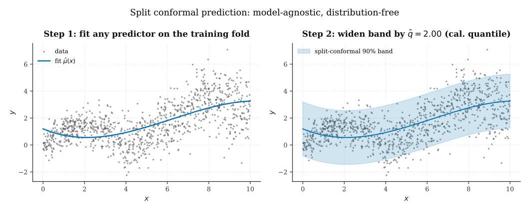
The left panel shows a cubic polynomial fit to half the data; the right panel shows the fixed-width band of radius $\hat{q}$ (the calibration quantile) around it. The band is not parametric. It is not the confidence interval of any model. It is the empirical answer to “how far off was the model on the calibration set, in the worst of the well-behaved cases?”, an answer that carries a finite-sample coverage guarantee automatically.

3. Marginal versus conditional coverage, the crucial caveat

The guarantee in (1) is marginal: the probability is averaged over $X_{n+1}$. This is not the same as a conditional guarantee

$$\mathbb{P}(Y_{n+1}\in {\hat{C}}_{\alpha }(X_{n+1})|X_{n+1}=x)\ge 1-\alpha \text{for all }x,(2)$$

which would say that the coverage holds for every covariate value.

Consider a bimodal data distribution with an “easy” group where $Y$ is near-deterministic given $X$ and a “hard” group where $Y$ is high-variance given $X$. A fixed-width split-conformal band can achieve 90% marginal coverage by over-covering the easy group and under-covering the hard group:

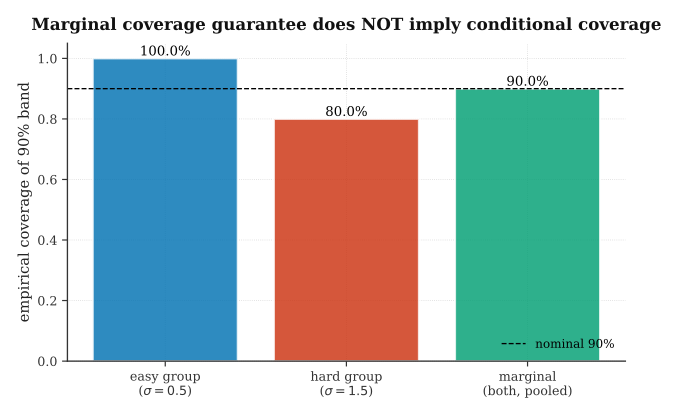
An impossibility theorem. Barber, Candès, Ramdas & Tibshirani (2021) proved that exact conditional coverage (2) in a distribution-free sense is impossible with finite data. Formally: any method that achieves (2) at some $\alpha >0$ for all distributions must produce sets that are trivially wide (covering $\mathcal{Y}$ almost always). Something must give. The three usual relaxations:

• Keep marginal coverage, accept that conditional coverage varies.
• Assume smoothness of the underlying distribution, trade distribution-freeness for approximate conditional coverage.
• Weaken to approximate finite-sample coverage with asymptotic conditional guarantees.

Conformalized quantile regression picks the second: it targets approximate conditional coverage by using a model that already produces approximately conditional intervals.

4. Conformalized quantile regression

Romano, Patterson & Candès (2019) proposed conformalized quantile regression (CQR). The idea: fit two quantile regressions ${\hat{Q}}_{\alpha /2}(x)$ and ${\hat{Q}}_{1-\alpha /2}(x)$ on the training fold; the base interval is $[{\hat{Q}}_{\alpha /2}(x),{\hat{Q}}_{1-\alpha /2}(x)]$; conformalize this interval by adjusting its width based on calibration-set residuals.

The nonconformity score is

$$s(x,y,\hat{\mu })=\max ({\hat{Q}}_{\alpha /2}(x)-y,y-{\hat{Q}}_{1-\alpha /2}(x)),$$

which is positive when $y$ is outside the base interval and negative when $y$ is inside.

The calibrated interval is

$${\hat{C}}_{\alpha }(x)=[{\hat{Q}}_{\alpha /2}(x)-\hat{q},{\hat{Q}}_{1-\alpha /2}(x)+\hat{q}]$$

where $\hat{q}$ is the calibration quantile of $s$. When the quantile-regression model is well-calibrated, $\hat{q}$ is near zero; when the model over- or under-predicts the interval width, $\hat{q}$ corrects for it. The marginal coverage guarantee (1) is preserved by the exchangeability argument; the approximate conditional coverage comes for free whenever the quantile regression captures the heteroscedasticity structure.

4.1 CQR vs. fixed-width conformal on heteroscedastic data

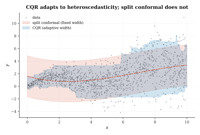
On heteroscedastic data (noise variance grows with $x$), split conformal pays the cost of the worst-case point: the band is wide everywhere. CQR adapts, the interval is narrow where the quantile model says it should be narrow, wide where the model says it should be wide. Both achieve the same 90% marginal coverage guarantee; CQR does so with smaller interval sizes on easy inputs and larger intervals on hard inputs. This is the “approximate conditional coverage” property, and it is what makes CQR the default production choice.

5. Adaptive conformal inference under distribution shift

Exchangeability is a strong assumption. In online or streaming settings, recommender systems, weather forecasting, spam detection, the data distribution shifts over time. The exchangeability argument fails; the conformal coverage guarantee fails with it.

Adaptive conformal inference (Gibbs & Candès 2021) parameterizes the method by a rolling target miscoverage rate ${\alpha }_t$ and updates it based on whether coverage failed at step $t$:

$${\alpha }_{t+1}={\alpha }_t+\gamma ({\alpha }^{\ast }-1[\text{miscovered at }t]),(3)$$

where ${\alpha }^{\ast }$ is the user’s target miscoverage rate and $\gamma >0$ is a step size.

• If the method miscovered at $t$ (indicator = 1), (3) decreases ${\alpha }_t$, driving the effective threshold toward keeping more scores, producing a wider interval at $t+1$.
• If it covered correctly (indicator = 0), (3) increases ${\alpha }_t$, producing a narrower interval at $t+1$.

Theorem (Gibbs & Candès 2021). The long-run miscoverage rate converges to ${\alpha }^{\ast }$ for any data sequence and any prediction model, with no distributional assumptions whatsoever.

The tradeoff: the guarantee is long-run, not pointwise. Under a violent distribution shift the adaptive method will be under- or over-covering for some number of steps before correcting. The explicit compensation for distribution-freeness is that coverage is guaranteed over time rather than on every step.

6. LLM and agent applications

Conformal prediction has become the default method for principled uncertainty quantification in LLM outputs.

Calibrated generation. Wrap the per-token probabilities from an LLM with split conformal to produce a set of candidate completions that contains the true completion with specified probability. Used in safe code generation and factual QA.

Agent output reliability. The agent’s final answer is wrapped in a conformal set. If the set is small (low uncertainty), output directly. If the set is large, defer to a human reviewer or take a conservative fallback action. This is a principled way to operationalize the “augmentation, not replacement” posture discussed in the LLM agents note.

Anomaly and out-of-distribution detection. Unusual inputs produce large conformal sets, serving as a distribution-shift alarm. The marginal guarantee gives you an explicit Type-I error rate on the alarm system.

7. Three real-life applications

Medical imaging. Classifying chest X-rays with conformal prediction sets, patients whose conformal set contains multiple diagnoses are triaged to a radiologist. The Angelopoulos-Bates tutorial (2021) works through this example on the public MIMIC-CXR dataset.

Financial risk. Portfolio value-at-risk calculations with distribution-free coverage. Conformal methods are gaining traction in regulated environments because the coverage guarantee is auditable in a way that Monte Carlo or parametric VaR is not.

Weather forecasting. Post-hoc calibration of ensemble forecasts to achieve exact marginal coverage of precipitation intervals, without assuming a distributional form for the ensemble spread.

8. Open questions

Conditional coverage with practical usefulness. The Barber-Candès-Ramdas-Tibshirani impossibility is definitive, but practical approximations (CQR, locally-adaptive conformal, group-conditional conformal) are incomplete. The right level of approximation for a given application is not well-understood.

Structured outputs. Conformal prediction for graphs, sequences, molecules, and program code is under-developed. The nonconformity score must be designed carefully for each structure.

Conformal causal inference. Lei & Candès (2021) give early results on conformalizing counterfactual and individual-treatment-effect estimates; the field is young and the guarantees are weaker than in the i.i.d. prediction case.

Online conformal under abrupt shifts. Adaptive conformal handles smooth drift but has poor transient behavior under sudden distribution changes. Change-point-aware extensions are an active area.

9. References (verified April 2026)

• Vovk, V., Gammerman, A., & Shafer, G. (2005). Algorithmic learning in a random world. Springer.
• Angelopoulos, A. N., & Bates, S. (2021). A gentle introduction to conformal prediction and distribution-free uncertainty quantification. arXiv. [S.S. c3ea8eb8]
• Angelopoulos, A. N., Barber, R. F., & Bates, S. (2024). Theoretical foundations of conformal prediction. arXiv. [S.S. d2ae8e11]
• Papadopoulos, H., Proedrou, K., Vovk, V., & Gammerman, A. (2002). Inductive confidence machines for regression. ECML.
• Barber, R. F., Candès, E. J., Ramdas, A., & Tibshirani, R. J. (2021). The limits of distribution-free conditional predictive inference. Information and Inference, 10(2), 455–482.
• Romano, Y., Patterson, E., & Candès, E. J. (2019). Conformalized quantile regression. NeurIPS.
• Gibbs, I., & Candès, E. J. (2021). Adaptive conformal inference under distribution shift. NeurIPS.
• Lei, L., & Candès, E. J. (2021). Conformal inference of counterfactuals and individual treatment effects. JRSS-B, 83(5), 911–938.
• Tibshirani, R. J., Barber, R. F., Candès, E. J., & Ramdas, A. (2019). Conformal prediction under covariate shift. NeurIPS.

---

Figures produced by reproducible Python scripts in the site repository. Illustrative examples use small synthetic datasets; the methods scale to any data size with no change in the guarantee.